The components of the SDDA are:
An application partitions its N-dimensional problem domain into a finite number of regions. Each region can be associated with a unique coordinate in the problem domain. A discretization of these coordinates yields a finite set of N-dimensional indices within an N-dimensional index space.
Such an N-dimensional index space can be mapped to a 1-dimensional index space. A well known family of such maps are known as space-filling curves [11][10][9][8][7]. This mapping is used to fully order the finite set of N-dimensional indices associated with an application's partition of the N-dimensional problem domain.
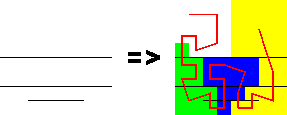
Figure 2, Space-Filling Curve Ordering of a Partitioned Domain, illustrates this process for an irregularly partitioned two dimensional problem domain. In this illustration a Hilbert space-filling curve is used to fully order the subregions. This particular space-filling curve has the property that points which are local along the one-dimensional curve map to points which are local in the N-dimensional space. This locality preserving property of the mapping is an essential feature of an application's configuration of the SDDA via the hierarchical dynamic index space.
Figure 2:
Space-Filling Curve Ordering of a Partitioned Domain
The space-filling curve maps have a recursive property, known as self-similarity, which leads to a computationally efficient implementation of the map. The level of recursion in a space-filling curve's map directly corresponds to a discretization granularity for the N-dimensional problem domain. Thus both the 1-dimensional and N-dimensional index spaces are hierarchical, and dynamic as the application can vary the map's level of recursion, or granularity, at run-time.
Once an application has defined an index space the application may easily partition its problem among processors by simply partitioning the index space. The color (or shade) coded regions in Figure 2 denote a partitioning of the problem geometry among four processors. This problem partitioning is easily and efficiently obtained by partitioning the 1-dimensional index space such that the computational load of each partition is roughly equal. Note that this approach, by virtue of the locality preserving property of the space-filling curve, results in a ``good'' partitioning of the problem.
The SDDA provides a storage structure, derived from extendable hashing [13][12], which provides storage locality for an application's data objects which are assigned local indices in the index space. Thus the ``array'' semantics where index locality implies storage locality.
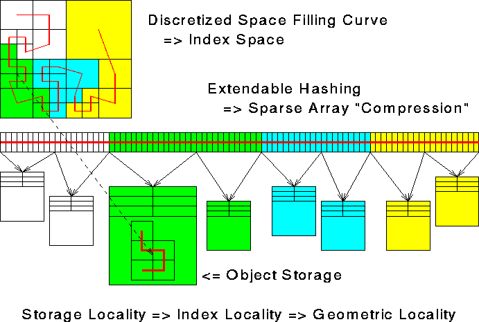
Figure 3: Locality Preserving Property
Figure 3, Locality Preserving Property, illustrates the end-to-end locality preserving property of the SDDA when configured with an index space derived from a space-filling curve. An application assigns indices to subregions via the space-filling curve mapping. The SDDA stores objects within a span of indices in contiguous blocks of memory, as illustrated. Thus subregions which have locality in the appliation's problem domain have locality in their associated data object's storage.
Recall that the application's partitioning of the index space defined a partitioning of the application's problem among processors. This index space partitioning also defines a distribution of the application's data objects among processors. The SDDA automatically distributes the application's data among processors, as illustrated by the color (or shade) coding of data storage blocks in the above illustration. The SDDA then provides global access to the application's data by transparently caching these storage blocks between processors.
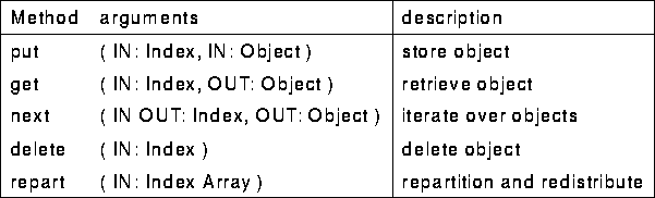
The SDDA interface consists of a simple set of methods. These simple methods, as denoted below, hide the complexity of the storage structure and make transparent any required interprocessor communication.
Two aspects of SDDA performance are evaluated: 1) time required for local put/get operations and 2) time required for interprocessor caching. The performance of these operations is dependent upon the computational environment, the SDDA's storage block size, and the size of the application's data objects. The performance results presented here where obtained from a network of RS6000/3BT workstations using the MPICH communication library from Argonne National Labs.
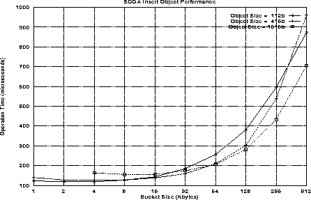
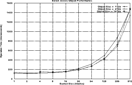
Figures 4 and 5 illustrate the overhead associated with inserting and deleting objects in the SDDA. These results were obtained by inserting 5000 objects with random indices into a single processor SDDA and then deleting all 5000 objects. These operations introduce two overhead costs: 1) inserting/deleting the object from a storage block and 2) dynamically expanding and contracting the set of storage blocks. Thus the per-operation cost includes an amortization of the storage expansion/contration performed periodically during the 5000 inserts and deletes.
Figure 4: SDDA Insert Object Performance
Figure 5: SDDA Delete Object Performance
The data object size and storage block size are varied to determine their effect on SDDA performance. The overhead cost of inserting and deleting is dominated by the storage block size. This is an expected result as larger storage blocks require greater memory movement for expansion and contraction of the SDDA's storage. The ``acceptability'' of this overhead is a function of the work performed with an object. Each data object stored in the SDDA should have a sufficient lifetime and data content to acceptably amortize its creation and deletion overhead.
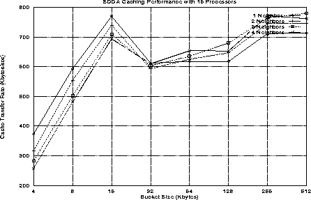
Figure 6 illustrates the data transfer rate of the SDDA's interprocessor data caching mechanism. Interprocessor data caching occurs through a pair of asynchronous request and reply messages. Interprocessor caching is unscheduled, any processor may request data from any other processor at any time, thus the performance experiment varies the number of processor ``neighbors'' from which data is simultaneously cached.
Figure 6: SDDA Caching Performance
As seen in Figure 6 the transfer rate improves with bucket size, up to a start-up versus bandwidth limit. An additional argument for modest size buckets is that a large bucket will likely contain numerous data objects which are not needed on the remote processor. Thus more data is transfered than is actually needed.