Blackbody Radiation
The phenomenon investigated in this experiment was blackbody radiation.
A lightbulb was used to assimilate a blackbody, and current and voltage
measurements were taken, from which, all other quantities, namely temperature and resistivity, were determined. The value for the Stefan-Boltzmann constant for tungsten was determined to be 2.743814512 x 10⁻⁸ which differs from the Stefan-Boltzmann constant of a perfect blackbody by approximately 51%. This difference is to be expected since tungsten behaves as a greybody, not a blackbody. The plot of power emitted versus temperature to the fourth power reveals a linear relation (for tungsten), thus confirming the Stefan-Boltzmann Law. Contained in the following paper is also a very detailed theoretical section which explains why the quantum hypothesis is necessary. This section is by no means necessary for the general development of the interpretation of this experiments results, however it was added for the purpose of giving a more rigorous explanation to Planck’s hypothesis, and also to aid myself, the author of this paper, in understanding the fundamental details at work.
Introduction
And God said, "A system of bodies of arbitrary nature, shape, and position which is at rest and is surrounded by a rigid cover impermeable to heat will, no matter what its initial state may be, pass in the course of time into a permanent state, in which the temperature of all bodies of the system is the same. This is the state of thermodynamic equilibrium, in which the entropy of the system has the maximum value compatible with the total energy of the system as fixed by the initial conditions. This state being reached, no further increase in entropy is possible." Actually this is the statement of the second principle of thermodynamics. It was from this statement that came the birth of quantum mechanics. Well, sort of.
Quantization in nature was not known in the 19th century. It was thought that macroscopic reality may be made up of microscopic quantities, but there was no proof. This idea however was used to develop the kinetic theory of gases, and was eventually found to be true. Another form of quantization was also known, quantization of the electric charge, which was discovered by pioneers such as Robert Milikan and Michael Faraday. These examples of quantization in nature however did not facilitate the necessity to develop a new theory of physics. The revolutionary step came in 1905 when Max Planck announced that energy must be quantized. This announcement basically said that motion was quantized in radiation and matter. The idea that the energy of a system could exist only in discrete states was not taken well by the physics community, but it was on this idea that the foundation of the new physics was built.
The downfall of the classical theory was partially due to its attempt to explain how radiation interacts with matter. Imagine an object that is either a perfect absorber or perfect emitter of radiation. A fairly good, in lab, example of a blackbody can be made with a box that has a small hole in the side. As this blackbody is heated, one can look at the radiation that is emitted from a small hole in the side. As the temperature is increased, the frequency of the radiation being emitted increases (thus the wavelength decreases). On a graph of wavelength versus luminosity (power per area), as the temperature is increased, the peak of the emitted radiation shifts from right to left.
The problem is that the best classical theory predicted that as the temperature increased (corresponding to an increase in luminosity toward the ultraviolet spectrum), the box full of radiation should have an infinite amount of energy. This did not agree with experiment, since there is a peak in the blackbody spectrum, and then it falls away to zero at short wavelengths (see picture below). According to classical theory, the energy should go off the scale at the short wavelength end. This was known as the Ultraviolet Catastrophe. This pointed out that there was definitely something wrong with the classical picture, at least with its predictions for energy at short wavelengths.
The classical theory’s predictions are in accordance with observations for the long wavelength spectrum (i.e. when the frequency is low, which corresponds to a lower temperature). That expression is known as the Rayleigh-Jeans formula, and its predictions agree with experiment for very long wavelengths. Another law, known as Wien’s Law, correctly predicted that the energy in an oscillator would go to zero as the wavelength decreased (on its radiation spectrum). Wein’s formula provided the correct solution when the emitted radiation was at very small wavelengths, but Wien’s formula showed small deviations from experimental values at large wavelengths. Thus there existed two classical formulas that predicted parts of the observed radiation spectrum, but no single formula that could encompass it all.
Enter Max Karl Ernst Ludwig Planck. Max Planck was a physicist of the "old school". This implied that he was a solid defender of the classical laws. Planck’s specialty was thermodynamics, and it was with thermodynamics that Planck thought he could tidy up the ultraviolet catastrophe. He began his work on the problem in 1895. For the first five years, he published many papers that connected thermodynamics to electrodynamics, but he still could not find an answer to the catastrophe problem. His first big break came in 1900. He struggled to explain the ultraviolet catastrophe and in desperation after some mathematical manipulation, he found an expression that agreed with the physical observations. This new expression however, had absolutely no physical basis, and most physicists of the time saw Planck as nothing more than a ‘mathemagician’.
Planck, for the next few months, immersed himself in trying to find a physical basis for the mathematical description. After exhausting all his options, he arrived at the alternative that most disturbed him.
Returning to the idea of Planck as an "old school physicist" for a moment, one must realize that this meant that he did not welcome the statistical interpretation of thermodynamics.
Enter Ludwig Boltzmann. Boltzmann made many contributions to physics. One of those contributions was that he (and Josef Stefan independently) deduced from thermodynamics that the power per area radiated by any object was proportional to the fourth power of the temperature (of that object). This relation is known as the Stefan-Boltzmann Law. Boltzmann was excellent with statistics. He used them to interpret thermodynamics, and argued from this point of view that it was possible for a decrease in entropy, although not very probable. "His statistical approach to thermodynamics involved cutting up energy into chunks, mathematically, and treating these chunks as real quantities that could be handled by the probability equations." This energy would normally then, be recombined by integration to give back the total energy. Planck took Boltzmann’s approach to thermodynamics, reluctantly, and attempted to use this method to attack the blackbody problem. In applying this method, Planck realized that before the step of integration, he had a formula for the blackbody spectrum.
Mathematically, he should have integrated, but since he knew what he was looking for, he stopped short.
Enter Albert Einstein. Einstein is responsible for correctly interpreting Planck’s results in terms of quanta. He also showed how integrating Planck’s formula would have led back to the ultraviolet catastrophe, as would any classical approach to the problem. This new realization of discrete energy states had tremendous ramifications for physics. An entirely new theory of physics had to be developed.
Thus, the focus of this paper will be to develop the theoretical background (both classically and quantum mechanically) of blackbody radiation, and to show how one arrives at energy quantization, and Planck’s formula for the spectrum of radiation of a blackbody. The data analysis section will present experimental verification of the Stefan-Boltzmann Law. This law can be derived from Planck’s formula, thus by validating the Stefan-Boltzmann Law, I will be indirectly verifying that energy quantization is the correct interpretation for physical reality.
Theory
An ordinary property of all matter is its ability to emit and absorb electromagnetic radiation. This phenomenon is called thermal radiation. It is called thermal radiation because it involves an exchange between radiation energy in the electromagnetic fields surrounding an object, and thermal energy caused by the motion of particles within an object. This interchange is assumed to be an equilibrium process, and occurs at a specific temperature. If the temperature of the object changes, the radiation emitted changes frequency. This is obvious if one looks at a hot piece of metal. If it is red-hot, and the temperature is increased, it becomes white-hot. There is some relation between the temperature of an object, and the frequency of electromagnetic radiation that is emitted.
Classically, there was a problem describing the spectrum of radiation from an object in thermal equilibrium. The classical formula for the spectrum is given by the Rayleigh-Jeans formula, and it is derived in the following manner.
- Consider a hollow cavity whose walls are held at a fixed temperature. Assume that one of those walls has a very small hole in the side to allow the entrance of radiation. Any radiation that enters will presumably be absorbed before it has a chance to "bounce" out of the hole. The radiation inside the "blackbody" will, after some time, be in thermal equilibrium with the walls of the cavity, and so the energy inside is continually being absorbed and re-emitted by the walls. The energy that happens to escape (i.e. is reflected from a wall at an angle such that it exits through the small hole) will have the same spectrum as the radiation inside the cavity.
- Think again of a hot metal object. When the object glows bright red, it means that most of the radiation being emitted has a frequency corresponding to the red wavelength ~700 nm. When an object glows white, it means that most of its thermal spectrum occupies the visible region. Since all visible frequencies are being emitted (roughly at the same intensity), white light is observed (white is the composition of all visible frequencies super-imposed). When I say most of the radiation, I mean the peak in the radiation spectrum (see figure below). The reason it seems as though a hot piece of metal radiates only a small band of frequencies, is that we only see the portion of this metals emitted spectrum that lies in the visible range. The metal radiates at all frequencies however, there happens to be a dominant range, or peak, that occurs at a given temperature. Thus, the frequency of electromagnetic radiation being emitted can be described using a distribution that displays the power radiated per area per unit frequency versus the frequency (wavelength can be used instead of frequency since they are related by c = l
n
).
This distribution (as seen in picture above) is called the spectrum of the radiating object.
- In order to describe this spectrum, one needs to know how much energy per volume (in the form of radiation) is in the hollow cavity.
To find how much energy is in the cavity, start by counting the number of electromagnetic waves in the cavity:
This can be done by starting with the wave equation:
Where F(x,y,z,t) is a function describing the oscillating components of the electric and magnetic fields.
Assume a solution of the form:

with these boundary conditions:
F(0,0,0,t) = 0
F(L,L,L,t) = 0
These boundary conditions give rise to solutions that are purely standing waves:
In order to find the relation between the wavelength l
of these standing waves and the length L of the cavity (which is needed to count the number of standing waves), it is necessary to insert equation (2) above into equation (1). The relation obtained is given by:
Which can be simplified:
The number of modes that can be supported by this cavity can be found in the following way. Since this derivation is to lead to a general form for radiation of an object, where dimensions of the cavity do not matter, a simplification can be made. Let the cavity be a sphere that is centered in a Cartesian coordinate-space at (0,0,0), with coordinate axies labeled n1, n2, n3.
 If the values of n were allowed to be negative, then the total number of modes supported by the cavity would be equal to the volume of a sphere in the aforementioned n-space. Since negative values are not allowed however, the volume of the sphere must be divided by 8. Another aspect that must be considered is that there are two possible orientations of the electric and magnetic fields (i.e. polarizations), so a factor of two must be added for compensation. Thus the total number of modes that can be supported by this cavity is:

Where the radius is given by:
 But if instead of inserting equation (5) into equation (4), use the relation (3), and the number of modes in the cavity can be found in terms of the wavelength and the length of the cavity walls.
 Now the number of modes per unit wavelength can be obtained by differentiating (6) with respect to l
:
Now the number of modes per unit wavelength can be obtained by differentiating (6) with respect to l
:
The number of modes per unit wavelength per cavity volume can then be found by dividing (7) by the volume of the cavity (1/L3).
The next step will demonstrate, eventually, why the classical theory of heat radiation fails. Now that we have an expression for the number of modes per unit wavelength, it is necessary to find the energy per volume per unit wavelength. To find this, one must first determine what the average energy of each oscillator is. The average total energy of a wave for each degree of freedom is found to be kT (where k is Boltzmann’s constant, and T is the absolute temperature of the system, measured in kelvins). This is arrived at from the standpoint of classical statistical physics, and is a result of the application of the principle of equipartition of energy. The failure of the classical theory is now beginning to materialize. The energy per volume per unit wavelength is given by:
 Now the next step is to relate the energy in the cavity volume, (8), to the power per area per unit wavelength radiated from the surfaces of the walls of the cavity. For radiation that is normal to the cavity wall, the power radiated per area per unit wavelength is:
 The power radiated per area per unit wavelength that is not normal to the surface of a cavity wall is given by:
 So the total power radiated per area per unit wavelength is given by what is called the Rayleigh-Jeans formula. It is the classical formula for thermal radiation from a cavity and is stated:
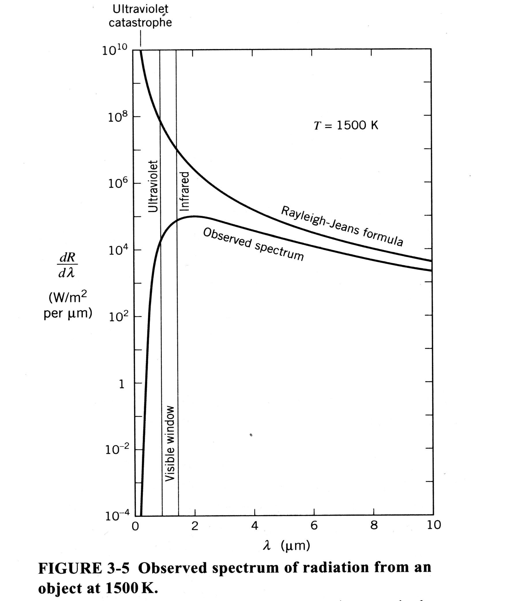 One important thing to note is that the power radiated does not depend on the dimensions of the cavity. It is also important to note that this expression gives rise to the ultraviolet catastrophe. This catastrophe is the fact that this formula predicts that the power radiated in the small wavelength region (ultraviolet region) of the spectrum, is infinite. This is impossible. The Rayleigh-Jeans distribution predicts a peak in the ultraviolet range, whereas experiments show the peak drops off to zero at small wavelengths.
 Obviously there was a problem with the classical picture, which needed to be fixed. A man by the name of Wilhelm Wien tried to solve the blackbody problem by hypothesizing a solution of the form:
 If a change of variables is performed, this distribution predicts a temperature to the fourth dependence on power radiated. This can be shown in the following way:
In equation (13), R is the total power radiated. This formula was almost perfect, but deviated slightly from experimental results at large wavelengths. The importance of this formula however, was that it correctly predicted that the power radiated was proportional to the fourth power of the temperature.
The next stage in the progress of solving this problem was made by Planck. This step is what ultimately led to the development of the quantum theory of physics. Planck hypothesized that the energy distribution of atomic oscillators in the wall of the cavity was not continuous. He said that the thermal spectrum of radiation could be explained if the spacing between energy levels that the oscillators could occupy was proportional to the frequency of oscillation.** This implied that the energy, En, should correspond to n multiples of a fundamental unit of energy, hn
, called a quantum of energy. Thus if:
 The difference between energy levels of the oscillators could be written as:
If an atom is oscillating at frequency f, and it gives off radiation at its oscillation frequency, then the wavelength of the radiation is:
 The reason that the idea of quantization can explain the radiation spectrum is simple. If the oscillators can assume any energy (i.e. a continuous distribution), then the average energy is kT. If however, the energy distribution is quantized, then at very high frequencies (small wavelengths), most of the oscillators are in the E0 state which corresponds to an energy of zero. Only a small number of oscillators occupy the first (n=1) energy state, and this number is proportional to e-hc/l
kT as will be shown momentarily.
The reason that the idea of quantization can explain the radiation spectrum is simple. If the oscillators can assume any energy (i.e. a continuous distribution), then the average energy is kT. If however, the energy distribution is quantized, then at very high frequencies (small wavelengths), most of the oscillators are in the E0 state which corresponds to an energy of zero. Only a small number of oscillators occupy the first (n=1) energy state, and this number is proportional to e-hc/l
kT as will be shown momentarily.
Now that it has been assumed that these atomic oscillators occupy only discrete energy levels, the average energy per oscillator must be recalculated. The distribution function that describes how the energy is distributed among oscillators is a discrete function:
The average energy per oscillator is given by:
This can be solved by a simple change of variables. Let x = hc/l
kT, and y = e-x.
The denominator of (14) can be rewritten as:
 And the numerator can be simplified by noticing that:
 So that the sum in the numerator can be written as:
 So (14) can be solved, and upon recombining (15) and (17), it yields:
Now, that the average energy has been determined for atomic oscillators with
 consideration for energy quantization, the ultraviolet catastrophe is ready to be cleared up. Return to equation (11), and insert the newly found average energy in place of the old value kT. This gives:
This equation correctly predicts the radiation spectrum emitted from an object in equilibrium at a set temperature. Thus, the ultraviolet catastrophe is resolved. From this distribution, the total power radiated per area can be found by integrating (19) over all wavelengths:
Where s
is the Stefan-Boltzmann constant and it equals 5.67 x 10⁻⁸ W. m-2 . K-4 .
This relationship (20), is the relationship that is to be confirmed for our experiment. Note however, that this relationship is derived for a perfect blackbody, which of course, tungsten is not. Therefore, some relationship must be developed to relate the spectral radiation observed for tungsten (or, in general, any object) to the distribution observed from a perfect blackbody. Thus definitions must be introduced.
 An important quantity that can be used to describe the blackbody phenomenon is radiant emittance. This is defined as the total energy radiated by an object at Kelvin temperature T per unit time per unit area, and is denoted M(T) (which is equivalent to the above notation of (dR/dl
)). Since this radiant emittance has frequency contributions in every interval dn
, a continuous wavelength spectrum is defined. This distribution can be written as:
An important quantity that can be used to describe the blackbody phenomenon is radiant emittance. This is defined as the total energy radiated by an object at Kelvin temperature T per unit time per unit area, and is denoted M(T) (which is equivalent to the above notation of (dR/dl
)). Since this radiant emittance has frequency contributions in every interval dn
, a continuous wavelength spectrum is defined. This distribution can be written as:
The integrand Mn
(T) is what is called the spectral radiant emittance. This differs from the radiant emittance in that it is the total energy radiated per unit time per unit area per unit frequency interval, which is totally dependant on only the frequency and temperature.
In order to be able to describe real objects (not ideal), some ideal object must be defined. This ideal object is known as a blackbody. Its characteristics are that it is a perfect emitter and absorber of radiation. In order to quantify this statement, more definitions must be made and used.
For a body in equilibrium, energy absorption and emission occur at the same rate. If radiation is incident on an object, it can either be absorbed or reflected. Thus a spectral absorptance a
l
(T) and spectral reflectance r
l
(T) must be defined. It seems obvious that the sum of absorptance and reflectance would be one, and so:
a
l
(T) + r
l
(T) = 1.
The ratio of Mn
(T)/a
n
(T) was proved to be a universal constant by G.R. Kirchoff in 1859.
Getting back to the ideal blackbody, it follows from the previously mentioned definition that a
l
(T) = 1, which says that a blackbody’s spectral absorptance equals one. This makes sense because a blackbody is an object that absorbs all radiation incident upon it.
Now that we have somewhat of a definition of a blackbody, we can define a quantity which will allow for the description of real objects. This quantity is called the spectral emissivity:

In this equation, Mn
b denotes the spectral radiant emittance of the previously defined ideal object, a blackbody. The relation between spectral radiant emittance in terms of frequency, and that in terms of wavelength is:
Thus we now have a way of dealing with non-ideal, graybodies, and can proceed to analyze the problem.
A theoretical value of the Stefan-Boltzmann constant can be determined (and verified with our experimental data) in this manner:
So when calculating the power radiated per area for tungsten, replace Ml
b in the integral, with the expression for Ml
above. The new spectrum is:
 Where s
’ is the Stefan-Boltzmann constant for a greybody whose value will be determined in the data analysis section.
Where s
’ is the Stefan-Boltzmann constant for a greybody whose value will be determined in the data analysis section.
Appendix (for theory section):
This discussion here is in no means necessary, however I became so enthralled while studying the blackbody radiation problem, and the introduction of quantum ideas, that I thought to include it to facilitate my own knowledge of how Planck’s ideas of quantization came about, by trying to transfer them to this document in my own words. A majority of what is in here is paraphrased from Max Planck’s book, The theory of heat radiation. Below is Planck’s description of how entropy and probability give rise to a hypothesis of quanta.
Probability is unrelated to the fundamental principles of the theory of electrodynamic heat radiation. Therefore, if probability is to be considered in the theory of heat radiation, its considerations must be justifiable and necessary.
Probability’s entrance into electrodynamics is both justifiable and necessary by considering the dilemma that exists between what is meant by "initial/boundary conditions and how a process evolves in time" in thermodynamics versus what is meant by the same statement in electrodynamics. Consider the case of radiation in a vacuum that is uniform in all directions. Thermodynamics says that once the intensity of radiation is known, the state of the radiation is completely determined. It also says that the systems evolution in time is determined by the constancy of the amplitude of the radiation. Electrodynamics says however, that the determination of the state of the radiation requires that every component of the electric and magnetic field strengths must be given at all points of the occupied space. The evolution, electrondynamically speaking, is determined by knowledge of the amplitudes and phases of all of the components.
The problem arises because data obtainable by measurement is by no means sufficient to meet all of these electrodynamic demands.
The thermodynamic values obtained represent only mean values (as seen by an electrodynamicist). Therefore, an electrodynamic state is not determined by thermodynamic data because particular values (those corresponding in this case to the components of E and B-field) can not be obtained from mean values. This implies that electrodynamic theory fails in cases where a completely unambiguous result is to be expected, since "It allows not one definite result, but an infinite number of different results."
To find how thermodynamic processes evolve in time, it is sufficient to determine initial and boundary conditions. By doing this, one finds a solution to the evolution of the system that is unambiguous (that is, there is a unique solution).
Determining the initial and boundary conditions is not sufficient however for electrodynamically determining the behavior of the system, because as stated above, there are far too many conditions to be actually (experimentally) obtainable. Mean values must be used. Therefore, this gives rise to an infinite number of results, some of which defy the second law of thermodynamics.
If one wishes to keep the possibility of determining thermodynamic processes electrodynamically, the initial and boundary conditions must be supplemented with special hypotheses. These hypotheses must cause the electrodynamic equations to lead to an unambiguous result that agrees with experience.
These hypotheses must now be determined. As to how this hypothesis is determined, no hint can be taken from the principles of electrodynamics, because they leave this question entirely open. On that note, the hypotheses are therefore admissible a priori. Thermodynamics lends itself to the determination by considering the following example.
Consider a flowing gas. The mechanical or electrodynamic state of all the separate molecules is not defined by the thermodynamic state of the gas. If however, all possible combinations of the position and velocity of the separate molecules, consistent with given values of velocity, density, and temperature, are considered, and all of the mechanical (or electrodynamic) processes are calculated for each combination, one will arrive at processes that agree with the mean value for most considerations. The cases which deviate appreciably (non-ordinary experience) from the mean values, only occur when "very special" conditions between the position and velocity exist. Therefore, if one assumes that these "very special" conditions do not exist, a form of flow of the gas will be found which will be definite with respect to all mean values, and these forms are the only ones which can be determined experimentally. "And the remarkable feature of this is that it is just the motion obtained in this manner that satisfies the postulates of the second principle of thermodynamics."
From the consideration of this example of a flowing gas, the hypotheses, whose introduction were proven above to be necessary (in order to still use electrodynamics to obtain a theory of heat radiation), fill their purpose if they do nothing more than state that "very special" conditions do not exist in nature.
Any condition for which such a hypothesis holds can be described as an "elemental chaos"*. This elemental chaos furnishes the necessary condition for a unique determination of the measurable processes in mechanics and electrodynamics, as well as for the validity of the second law of thermodynamics.
Elemental chaos is the electrodynamical equivalent explanation of entropy. Entropy is a characteristic of the second law of thermodynamics, and is closely tied in with temperature. This implies also that the significance of entropy and temperature are associated with the condition of an elemental chaos.
Consider a periodic plane wave. The terms ‘entropy’ and ‘temperature’ do not apply to a periodic plane wave since all quantities in this wave can be measured independently. This implies that there exists no elemental chaos in this plane wave. The necessary condition for the hypothesis of elemental chaos (which implies that ‘entropy’ and ‘temperature’ exist) can consist only of the irregular simultaneous effect of many vibrations (from a wave) of different periods which propagate independently of each other. These conditions exist in the blackbody problem.
Now that elemental chaos has been introduced as the special hypothesis for the initial and boundary conditions of a system, and this chaos is intricately woven to entropy, a determination of what electrodynamical quantity represents the entropy of a state must be made.
Consider the following proposition:
The entropy of a physical system in a definite state depends solely on the probability of this state.
Let S denote entropy, and W denote thermodynamic probability. The above proposition states that:
S = F(W).
In this expression, F is a universal function of W. Here is the method to determine this function explicitly.
Mathematically, the probability of a system that consists of two entirely independent systems, is a product of the probabilities of these two systems.
Consider two systems:
The probability that the first system is in state 1, and the second system is simultaneously in state 2 is:
Wstate=(W1)*(W2)
Where W1 and W2 are the probabilities that the two systems involved are in the states in question.
If S1 and S2 are the entropies of the two states, then:
S1 = F(W1) and S2 = F(W2)
are the corresponding entropies, and according to the second law of thermodynamics, the total entropy is:
Stotal = S1 + S2
so
F(W1W2) = F(W1) + F(W2)
F can be determined by taking partial derivatives, first with respect to W1, and then with respect to W2. This yields:
 where W1W2 = W which is the probability of the two systems being in the aforementioned states simultaneously. To find explicitly the entropy of the two states, solve the differential equation above to determine F(W1W2). The resulting expression is:
S = k(log W) + constant {k is a universal constant}
This equation determines the general way in which entropy depends on thermodynamic probability.
S = k(logW)
Here the constant has been included in the value of W as a constant multiplier. This logarithmic connection was first determined by Boltzmann, but his
expression differed from the one directly above because he left an additive constant which leaves the value of W undetermined. Planck assigns a definite value to the entropy (S) which eventually leads to the hypothesis of quanta, as well as a definite law of distribution of energy of blackbody radiation, as we shall soon see.
W is the thermodynamic probability, which differs from mathematical probability in that mathematical probability is a ratio while thermodynamic probability is always an integer. The relation found above gives an explicit relation between thermodynamic probability and entropy, but is useless unless the value of W is determined numerically.
The determination of W is done in the following way:
First one must define what is meant when talking about the state of a system. "By the state of a physical system at a certain time we mean the aggregate of all those mutually independent quantities, which determine uniquely the way in which the processes in the system take place in the course of time for given boundary conditions. Hence a knowledge of the state is precisely equivalent to a knowledge of the ‘initial conditions’".
When talking about a state, it is useful to develop some ideas of statistical physics. The following is the derivation of the Maxwell-Boltzmann distribution*.
Imagine a collection of N particles distributed over discrete cells, each cell representing a different energy. Classical physics allows us to introduce distinguishing labels so that we can follow each of these particles as they are assigned to different energy cells. This absolute specification of the system is called a microstate. This description is unnecessarily complete since two microstates should be considered equivalent if their cell population numbers are the same without regard for the labels that distinguish the particles from cell to cell.
Another way of talking about states can be distinguished by introducing the notion of a macrostate. Imagine a list of numbers that specified how many particles were contained within each cell, regardless which particles were in that cell. That is, distribute N identical particles into r cells. Now, in the language of discrete and combinatorial mathematics, order does not matter.
Moving on, the hypothesis of ‘elemental chaos’ implies that all microstates are equally probable. Now it is obvious that a number of microstates can correspond to one macrostate. It can not be expected however that all macrostates will also have an equal probability of occurring. Thus, the number of ways to assemble a macrostate (from all the possible microstates), corresponds to the likeliness of that state existing.
The goal of all this is to develop an expression for the number of microstates corresponding to a given macrostate. Thus if the number of particles in an energy cell (energy cell is denoted Ä
n) is nr, then the thermodynamic probability, denoted WN(nr), of finding a given macrostate can determined by principles of counting.
 The number of unique ways to distribute N particles into r cells is:
*Note that in this section the equations used will be labeled with letters instead of numbers.
 Where WN gives the probability of finding a certain macrostate. Now that we have a relation for the number of ways to form a macrostate from N particles in r cells, we want to determine the most probable of these macrostates. The desired macrostate is the one that maximizes WN. Remember that entropy depends on logW, and note that the same distribution for is determined by the solution that maximizes logWN as opposed to WN. Thus, with no loss of generality:
 The expression (b) is obtained from (a) after a good deal of manipulation. Since a large number of particles are being used, some of the above quantities can be approximated with Sterling’s formula, thus:
 And now (b) becomes:
To maximize lnWN, we take integer increments in each ni, and seek the largest result. Since the increments we are talking about are so much smaller than the n’s themselves, it is reasonable to treat each ni as a continuous variable. Thus to obtain our solution we require:

 for every ni, if all the variables (n1L
nr) could all be regarded as independent. The problem is that only r-2 variables are independent. This is the case because of the conditions that the total number of particles, and the total energy of the system are respectively:
for every ni, if all the variables (n1L
nr) could all be regarded as independent. The problem is that only r-2 variables are independent. This is the case because of the conditions that the total number of particles, and the total energy of the system are respectively:
 Now there is a problem because not all of the variables are independent. This is not a catastrophe however, because a man by the name of J.L. Lagrange developed a way of dealing with this. Instead of using lnWN, a function of r variables (only r-2 of which are independent variables), introduce another function:
 where F is a function of r + 2 variables (all are independent). The procedure is then that we maximize F over all r + 2 variables, and we find the conditions:
so that the net effect is a maximization of lnWN, as required, while also satisfying the two constraints in (e).
 By combining (c) and (f), one obtains this expression:
 And so the maximizing condition in (h) becomes:
 where:
by using the left-hand side of (e), we can eliminate a
in this equation:

 where:
Here, Z is called the partition function. The expression (j) can then be rewritten as:
 which is the Maxwell-Boltzmann distribution. This formula specifies the number of particles in the ith energy cell for the macrostate of maximum thermodynamic probability. When a system approaches thermodynamic equilibrium, it approaches this configuration. Since the particles are continually rearranging themselves, this is not an absolute static solution, however large departures from the most probable thermodynamic macrostate are extremely unlikely.
 This is a very general form, where the partition function (l) depends on the manner in which e
i varies from cell to cell. Therefore, the value of b
must be determined for each case. There are an extremely large number of cases in which b
= (1/ kbT). Thus, with this assumption for the value of b
, the governing factor in the Maxwell-Boltzmann distribution is:
This is a very general form, where the partition function (l) depends on the manner in which e
i varies from cell to cell. Therefore, the value of b
must be determined for each case. There are an extremely large number of cases in which b
= (1/ kbT). Thus, with this assumption for the value of b
, the governing factor in the Maxwell-Boltzmann distribution is:
This expression gives the likelihood for the occurrence of a given energy e
in the distribution of energies in the cavity. The larger energies are suppressed by this function (n), and that leads to the following important result.
There is a comparison to be made between the Maxwell-Boltzmann distribution, and Planck’s hypothesis for the relation between energy and frequency (which says that the number of modes with a high frequency is very small). The Maxwell-Boltzmann distribution function was derived on mathematical grounds, as a problem in counting. It involved thinking of the allowable values of energy as discrete cells. The relation that Planck arrived at for the function of the blackbody spectrum was based on empirical results. These two statements are basically equivalent, and thus this implied that oscillating particles and radiation fields at frequency n
could exchange energy only in integral multiples of the quantum of energy, hn
.
In this development of the Maxwell-Boltzmann distribution, a split was taken from the explanation of the hypothesis of quanta in terms of entropy. I should now like to continue with that course, as it is more rigid and theoretically sound.
 Return to the expression (a) above which gave the thermodynamic probability of finding a particular macrostate. The numbers (n1,n2,. . . nr) for a cavity are obviously very large. Thus by applying Sterling’s Principle in a different manner, namely:
 a different form of the expression for thermodynamic probability can be obtained. This new form is:
 This expression, for the thermodynamic probability of a macroscopic state, (p), may be applied to all aspects of a problems parameters (i.e. the position, velocity, densities, etc). "Every thermodynamic state of a system of N molecules is, in the macroscopic sense, defined by the statement of the number of molecules, n1, n2, . . .,nr, which are contained in the region elements (energy cells) 1,2,3. . . of the ‘state space’." This state space is not required to be the ordinary three-dimensional space, but can occupy as many dimensions as there are parameters. The entropy of a state, with the above taken into consideration, is calculated in exactly the same way as mentioned earlier (S = klogW), but with also considering the statement:
where w
represents the mathematical probability (which can be thought of as a distribution density).
 The new expression for the entropy of a state is then stated as:
From the preceding developments, the calculation for the entropy of a system of N particles in a given thermodynamic state, is reduced to finding the magnitude of the region, or energy cell, in the ‘state space’. The idea that this region actually exists in a definite quantity is the basis of the quantum hypothesis.
This is the step where Boltzmann slipped up. Recall from earlier that Planck made a proposition that entropy had an absolute value, whereas Boltzmann defined entropy only to within a constant. This absoluteness of the value of entropy forces the value of thermodynamic probability to be defined absolutely. The thermodynamic probability (as developed above) depends on the number of microstates in the system, and also on the number and size of the energy cells which are used. Since all of the microstates contribute equally to the probability W, the energy cells of the state space also represent regions of equal probability. If this were not the case the microstates would not all be equally possible, but that condition is required by the hypothesis of ‘elemental chaos’. The necessity of the constancy of the energy cells can be demonstrated by considering the following argument. (Note that not only the magnitude of the energy cells, but also the shape and position must remain perfectly definite). If for instance the shape of an energy cell changed, the distribution density w
, which can vary drastically from one energy cell to the next, would change, and this change would lead to a change in the entropy S.
This leads to what is a very important aspect of the theory. Only when the distribution densities w
are very small can the magnitude of the region elements become physically unimportant. This arises because the magnitude of the cell enters into the value of entropy only as an additive constant. This occurs at high temperatures, large volumes, and slow vibrations. Thus, in the case of a hollow cavity, the classical picture works at long wavelengths because the magnitude of the energy cells is unimportant. The classical theory fails however when the energy cells assume any appreciable size. The preceding argument therefore provides, through considerations of probability and entropy, the necessity for the quantum hypothesis.
Apparatus
The experimental setup for this experiment was very primitive, and rather simple. This is a list of the only equipment used to obtain data:
- Two D.C.-Power supplies (connected in series)
- Two Multimeters: one for an accurate voltage measurement (parallel), and one for a current measurement (series)
- One tungsten-filament lightbulb (connected in series): it is the "blackbody" in the experiment
- Miscellaneous wires (both banana and alligator clip)
Circuit Diagram for apparatus:
PROCEDURE
The procedure for this lab was extremely straightforward. A potential difference was supplied by two sources of emf. The potential was varied in increments of 2.5 volts, and current readings were recorded. As the potential difference was increased, more power flowed through the lightbulb. Here was where the lightbulb failed to be a blackbody, and was instead a greybody. If it were an ideal blackbody, all of this power input (P=IV) would be absorbed, and radiated. Instead however, much of this power was dissipated by the filament and surrounding electrical devices, so the power input does not equal the power radiated by the filament. The values of potential and current were recorded, twenty times in 2.5 volt steps, in order to later determine the temperature of the filament, and thus the power radiated.
Data Analysis
 It was the purpose of this experiment to confirm the Stefan-Boltzmann Law which is stated symbolically as:
This relation states that the power radiated (by an object) per area per unit wavelength is proportional to the fourth power of the temperature of that object. By confirming this law, it will be equivalent to verifying Planck’s Quantum Hypothesis.
In measuring the potential applied to a lightbulb (containing a tungsten filament), and the subsequent current that flowed, the relation above could be found through a series of manipulations. From the measurement of current and voltage, the resistance could be obtained. The resistance is geometrically related to the resistivity. Once the value of resistivity was in hand, this value could be compared with national standards (which give tables of the resistivity of specific metals at certain temperatures) to obtain the temperature of the tungsten filament. This was done by making a plot of resistivity versus temperature, as given by the values in the national standards, and then by extrapolating the value of temperature directly from the graph. This was carried out for all of the values of resistivity. With this temperature now in custody, the power radiated by a perfect blackbody could be calculated.
The next phase was to determine the power radiated by a tungsten filament (which is not a perfect blackbody, it is more like a ‘greybody’). A plot of the emissivity of tungsten versus temperature was made, again using the values given by the national standards. The value of the temperature that was extrapolated from the graph above was then used to extrapolate the emissivity (at that particular temperature). This value of emissivity could then be multiplied by the power radiated from a perfect blackbody, and the power radiated by the tungsten filament would thus be obtained. To aid in the understanding of the procedure, I will include here a small flowchart of the method used.
Phase 1:
- Measure V (potential) and I (current)
- Calculate the resistance R from the above values (R = V/I)
- Calculate the resistivity r
from R (r
= R(A/l)
- Make a plot of resistivity versus temperature, using the values from the table of national standards
- Use the calculated value of resistivity (3) to extrapolate the temperature directly from the graph (4)
- Use this temperature (5) to calculate the power radiated by a perfect blackbody
Phase 2:
- Make a plot of the emissivity of tungsten versus temperature, using the values from the table of national standards
- Use the temperature obtained in (5) to extrapolate the particular values of emissivity from the graph (7)
- Multiply the value of emissivity (8) by the power radiated from a perfect blackbody (6) to obtain the value of the power radiated by tungsten.
This experimental value of the power radiated by a tungsten filament can then be
compared to the value radiated by a perfect blackbody, and the slopes of the two graphs can be examined. The slope of the power radiated by a perfect blackbody versus temperature to the fourth power, will yield the value of (s
)*(Asurface). When the slope is divided by the surface area of the filament, the Stefan-Boltzmann constant should be obtained. The slope of the power radiated from a tungsten filament versus temperature to the fourth power should yield the value of (s
tungsten)*(Asurface). This value, once the surface area is removed by division, will give the value of the Stefan-Boltzmann constant for tungsten. This value differs from that of a perfect blackbody because tungsten is not a perfect emitter of radiation. The value of s
tungsten is experimentally determined to be 2.743814512 x 10⁻⁸ W. m-2 .K-4 . This value differs from that of a perfect blackbody by 51.61%. This is to be expected since the average value of the emissivity of tungsten is 0.486. That means that the power emitted by tungsten is only about half of the power emitted by a perfect blackbody. The theoretical value of s
tungsten can be estimated if one  thinks of multiplying the average emissivity of tungsten by the known Stefan-Boltzmann constant. The theoretical value obtained in this way differs from the experimental value by roughly 0.523 %.
The most important thing to note about the graph of power radiated (for tungsten) versus temperature4, is that it is linear. This linearity confirms the Stefan-Boltzmann relation by demonstrating that the power radiated is (linearly) proportional to temperature to the fourth power.
The other graph that needs to be given attention to is that of the power supplied to the tungsten filament versus the power radiated from this filament. It is very obvious from the graph that power was dissipated in many ways, since the slopes of the graphs are not equal. This power dissipation will be dealt with in the next section.
Error Analysis:
It is in this section that I hope to account for all errors in the experiment, since a number of them exist. A large majority of these errors arise simply because only two quantities (namely voltage and current) are used to obtain all other values.
To obtain the error in certain values I did propagation of errors as follows.
The uncertainty in resistance (R=V/I) is:
 The uncertainty in resistivity (r
=R(A/l)) is:
The uncertainty in resistivity (r
=R(A/l)) is:
The uncertainty in the surface area of the filament (As=2p
rl) is:
 The uncertainty in the power radiated by the filament (Prad=Ass
T4) is:
The uncertainty in the power radiated by the filament (Prad=Ass
T4) is:
Where the uncertainty in T4 is given by:
 It should also be stated that the uncertainty in the value of the temperature T is equivalent to the uncertainty in the value of resistivity, since knowing the value of resistivity (for some value of current and voltage) is equivalent to knowing the value of the temperature (for those values of current and voltage) since temperature was obtained from tables. Therefore, in light of this consideration,

The uncertainty in the power radiated, is thus:
The numerical values of all of these uncertainties can be found in the raw data charts in the appendix. This uncertainty in the radiated power was used to weight the graph of the power radiated by tungsten versus temperature to the fourth power. The graph was weighted using a least squares method, which places more value on points with less uncertainty, thus giving the most accurate account of the data.
Above is an explicit account of all the errors in this lab that were accountable for numerically. Something that needs to be discussed however, are the errors for which no numerical solution can be accounted for. These errors arise with many faces, and I hope to exploit as many of them as possible, and to give a qualitative explanation as to how these errors affect the results.
One of the contributions to the error in the measurement of the power radiated can be attributed to a property known as thermal expansion. When an object is heated, it expands. In the case of the tungsten filament, this corresponds to an increase in surface area. Since the calculation of the power radiated per area by tungsten does not account for this increase in surface area, the calculated power (per area) is actually larger than the real value of the power (per area) being emitted. Another error comes in the form of electrical dissipation. This error arrives as a consequence of the wires being used in the experiment (to connect the power supply to the two multimeters and the lightbulb) having a resistance. The power supply delivers a constant potential to the lightbulb and causes a current to flow. Some of this current is dissipated by the wires before reaching the lightbulb, and the ammeter. This is a systematic error, and works to lower the value of the current, therefore raising the value of the calculated resistance, which causes an increase in the value of resistivity, which ultimately raises the value of the temperature that is used in the plot of power versus temperature (to the fourth power). This error is said to not be very large, but could still have small effects. Another error is contributed by the method in which temperature was obtained from the graph of resistivity versus temperature. A graph was plotted, using values of resistivity and the corresponding values of temperature. The values of temperature (at certain values of resistance) were then extrapolated directly from the graph. The calculated values of resistivity however, could not be matched up exactly with the values of resistivity from the graph, therefore the corresponding extrapolated temperature contained a small bit of fuzziness. This was not substantial, but could account for approximately a 0.8% deviation in the recorded value of the temperature. An error very similar to the one stated previously is also associated with the value of emissivity. This value was also extrapolated in the same manner as the temperature. Another error is that the purity of the tungsten was not known, and thus had to be estimated. This estimation involved calculating an average value of resistivity, which was used in the graph of resistivity versus temperature, which determined the value of the temperature of the filament. It can not be postulated as to how this averaging affected the results because the purity of the sample was not known. The calculation of the ratio A/l, which is used to determine resistivity (r
=(A/l)R), has an error because of its experimental nature. (A/l) was obtained by measuring the resistance of the filament at room temperature. This resistivity at room temperature was then divided by this resistance to arrive at a value for (A/l). This is a very erroneous method. In order to determine the resistivity, the multimeter sends a small current through the lightbulb. This current heats up the filament, and so its resistivity changes. Because of this and many other factors, the effect of this error is difficult to gauge.
Conclusion
From all of the experimental data, with considerations for the error as described above, it can be concluded that the Stefan-Boltzmann Law was verified for tungsten. The fact that the value of the Stefan-Boltzmann constant for tungsten differed from that for a perfect blackbody, gives rise to the conclusion that tungsten is not a perfect blackbody, but is rather a ‘greybody’. Further, by confirming the Stefan-Boltzmann Law, I inadvertently verified Planck’s quantum hypothesis on the grounds that the Stefan-Boltzmann Law is explicitly derivable from Planck’s more general law. This law predicts what the classical theory could not by considering fundamental units of energy, or quanta, in the description of the radiation spectrum observed from an object in thermal equilibrium.
Our experimental data concluded that the value of the Stefan-Boltzmann constant for tungsten is 2.743814512 x 10⁻⁸, which differed from the experimental value by approximately 0.523% as calculated by the method stated in the theory section of the paper. I must however, much like Max Planck, view this result with skeptical eyes. The reason I make this known is that I consider the method used for determining the theoretical value of this quantity unsatisfactory. Since so few variables were actually measured though, no other means were available to lend themselves to a more realistic theoretical value (if that statement isn’t loaded with oxy-morons). This being said, I would also like to add that it very possible, due to the magnitude of different sources of error in this experiment, that many errors worked together to, in effect, cancel each other out.
The methods I think that would contribute positively to improving the results of this experiment are two-fold. The first aspect I would change would be the method used in determining the value of the quantity (A/l). This method is very erroneous and could be improved by taking more measurements at room temperature, or by obtaining values from the manufacturer that would give complete a complete description of this variable, as it is difficult to gauge its magnitude in the laboratory. The second aspect I would change would be the number of independent variables measured. I would measure independently the emitted power with a gas-filled photocell, which has been found to experimentally provide good results due to the fact that it has a sufficiently large activation energy. This large activation energy is necessary because the infrared radiation in the thermal spectrum will dominate the obtained results if it is not somehow cut off. All this being said, I now lay the matter to rest.