More on SAMRAI and SUNDIALS for Black Holes

LIGO Gravitational Wave Detector in Louisiana

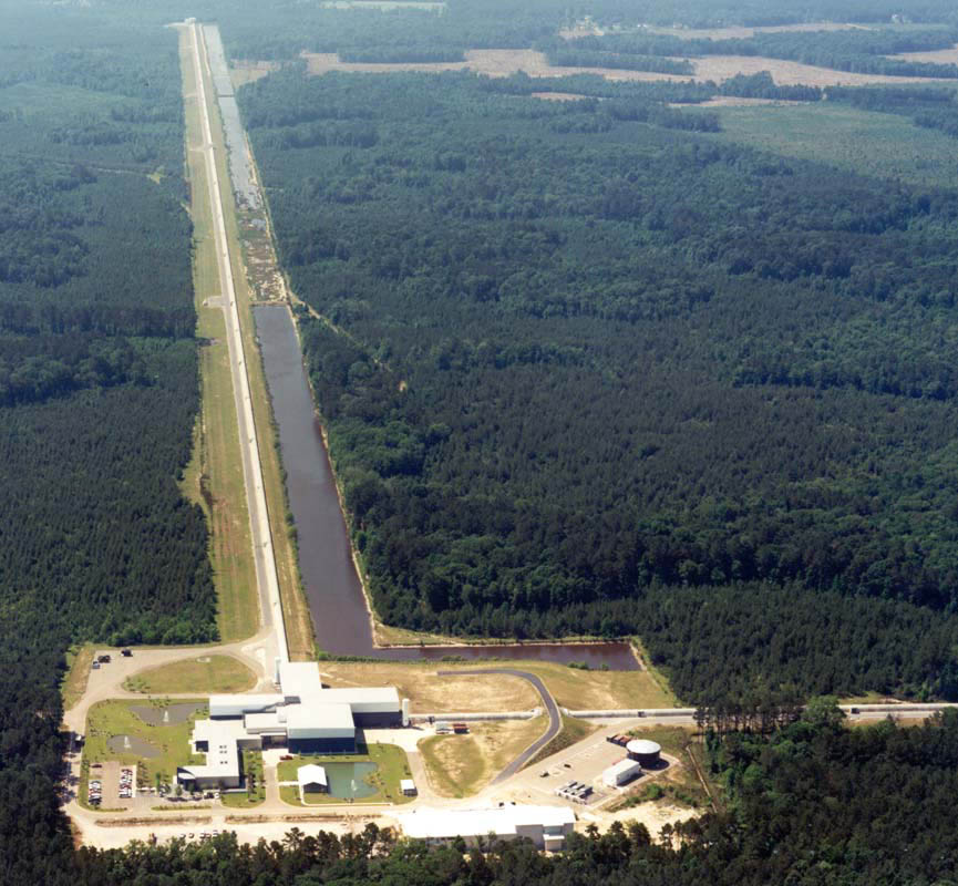
Black holes are the most likely candidates for detection by LIGO

Background:

Brian Gunney and the SAMRAI team requested that SAMRAI users keep the team informed of development successes. These pages are for that purpose.

The Problem:

The vacuum Einstein equations ( those appropriate to black hole physics ) constitute a constrained hyperbolic system. In three spatial dimenstions they are a set of six second order evolution equations and four coupled elliptic equations. The elliptic equations are generally called constraint equations.

Provided that the initial data of the evolution equations satisfy the constraint equations, the constraint equations analytically will be satisfied at all times. However, when solving the evolution equations numerically using analytic initial data ( e.g. like a single Schwarzschild black hole ) and simply monitoring the constraint equations ( unconstrained evolution ), constraint violating modes appear which cause the evolution to fail.

Such behavior will be familiar to those who conduct MHD simulations and monitor the divergence of the magnetic field. While it always should be zero, numerical simulations show violations unless care is taken to prevent it ( via constraint subtraction, constraint transport, or elliptic solves ).

An Approach:

Using KINSOL, part of the SUNDIALS package, I conduct elliptic solves every timestep on the constraint equations. This ensures that the constraint equations are satisfied and also promotes stability in the evolution.
Here is a plot of the constraint violations for a 1-D constrained evolution of an isolated black hole in Kerr-Schild coordinates compared with an unconstrained evolution:

In this large domain simulation (0.8M..150M) employing spherical symmetry with a resolution of 5pts/M the constraint violations are kept under control by the constraint solver while the unconstrained evolution oscillates and eventually blows up. While the symmetry certainly helps the simulation, similar behavior is seen in 3-D simulations as well.
Here is a plot of the constraint violations for a 3-D constrained evolution of an isolated black hole in Kerr-Schild coordinates compared with an unconstrained evolution:

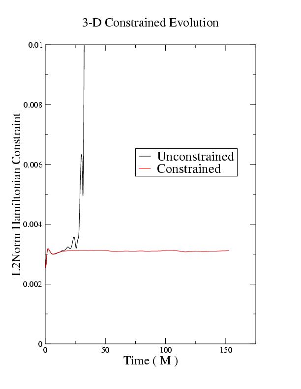These 3-D simulations were performed on a domain of -10M..10M and employ no special symmetries. The resolution was 5pts/M. The constraint solver keeps the constraints from blowing up and improves the stability of the simulation considerably. See gr-qc/0307055 for more details and other 3d results.

In order to model gravitational radiation, however, black hole simulations must not only be stable for very long times but also must be performed on very large computational domains ( reaching the radiation zone ). SAMRAI enables mesh refinement along with the special requirements of constrained evolution, enabling better use of limited computation resources.

Code Facts at a glance:

Uses Adams-Moulton for time integration ( via PVODE )

Uses Inexact Newton-Krylov method for elliptic solve ( via KINSOL )

All spatial finite differences are 4th order

Code is cell-centered

Solves full Einstein equations, both hyperbolic and elliptic parts

Utilizes mesh refinement in both the elliptic and hyperbolic solves

Uses standard ADM 3+1 decomposition of Einstein equations

Uses Kerr-Schild coordinates

Computation FAQ's:

I use the following packages, among others:
SAMRAI v1.3.1
PETSc 2.1.5
PVODE 18 Jul 2000
HDF5 1.6.0
ChomboVis 3.15.1

I have compiled SAMRAI with PETSc and SUNDIALS using:
gcc-3.2
xlC-6
icc-7.1

I found the xlC-6 compiler to be the most difficult to compile on. The others worked without difficulty.
I have notes on the compile process for xlC-6. Send me an email if xlC gives you trouble. Email: astro@einstein.ph.utexas.edu

I have now switched entirely from PETSc to KINSOL. However, here are some
notes about using PETSc 2.1.5 with SAMRAI-v1.3.1:

SAMRAI provides a vector class that can be used with PETSc. However, not all methods that PETSc uses are implemented.
This causes a failure in PETSc whenever the following commands are used:

VecNormBegin/End
VecDotBegin/End

To use SNES, you will likely have to replace the above with the commands:

VecNorm
VecDot

Check your PETSc documentation for more details.

For information on PETSc, see the PETSc home page for links and code

NOTE: This problem has been fixed in the newest version of SAMRAI when used with PETSc-2.1.6.

Notes on Excision

Numerically evolving the interior of a black hole is problematic due to the presence of the singularity. Further, the computational expense used in evolving the interior is wasted because the interior cannot causally affect the region exterior to the hole. We address this problem by excluding the singularity from the computational domain. This approach is called excision.

In short, we replace the singularity in the black hole with a mask function.

This grid is a 2-D slice from a 3-D single black hole evolution where the black hole is placed in the center of the domain. The blue shaded cells indicate points that have been masked in order to remove the singularity and the steep gradients immediately surrounding the singularity. The apparent horizon on the hypersurface is denoted by the red circle. Several evolved buffer points inside the apparent horizon but outside the mask are also shown.

The ``lego" shape sphere of the discretized mask function creates considerable difficulty for finite difference methods. 27 different 4th order difference stencils are used to evolve the inner boundary points. The inner boundary condition is free, made possible by the fact that the inner boundary is causally disconnected from the rest of the computational domain. Consequently, all derivatives next to the mask are ``one-sided".

Simulating isolated static black holes constitutes a demanding test problem with which to verify order convergence of a code. Evolving an isolated Schwarzschild black hole does not require adaptive mesh refinement ( no physical gravitational radiation in such case ). But fixed mesh refinement ( where the refinement region is around the black hole ) is extremely beneficial by reducing memory and computational costs for simulation.

Example of nested grids. This is a 2-D slice of the grid structure from a 3-D simulation employing mesh refinement. The fine local mesh is raised slightly above the coarse global mesh to reveal the overlap region between the two levels, indicated by the green square.

Notes on Interpolation

Interpolation occurs from the coarser level to the finer level in order to provide a boundary for the finer level.

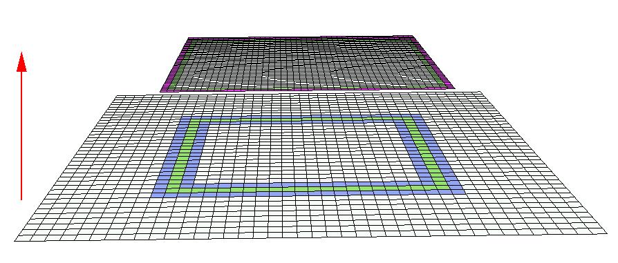Refinement step interpolation. The coarse and fine meshes are color coded to indicate how the refinement step interpolation proceeds. The green squares indicate the overlap region between the two levels. The arrow indicates the level where the interpolated values are copied to. The fine local mesh is displayed with one ghostzone, colored purple, which is filled with interpolated values from the coarse mesh points, colored blue and green.

Interpolation also occurs from the finer level to the coarser level in the region of the coarse-fine overlap.

Coarsening step interpolation. The coarse and fine meshes are color coded to indicate how the coarsening step interpolation proceeds. The green squares indicate the overlap region between the two levels. The arrow indicates the level where the interpolated values are copied to. Interpolation on the fine local mesh provides solution values to the coarse global mesh at points interior to a sphere contained inside the overlap region of the coarse and fine meshes. The purple disk on the coarse level indicates the destination of the interpolated values from the fine level.

When using adaptive mesh refinement, standard coarsening ( not spherical coarsening ) is employed outside the fixed mesh cube.

Notes on performance

Full performance measurements have not yet been completed. However, results from running large domain problems on different numbers of processors are available. The performance results so far observed are very promising. The memory benefits alone make the switch to mesh refinement worthwhile.

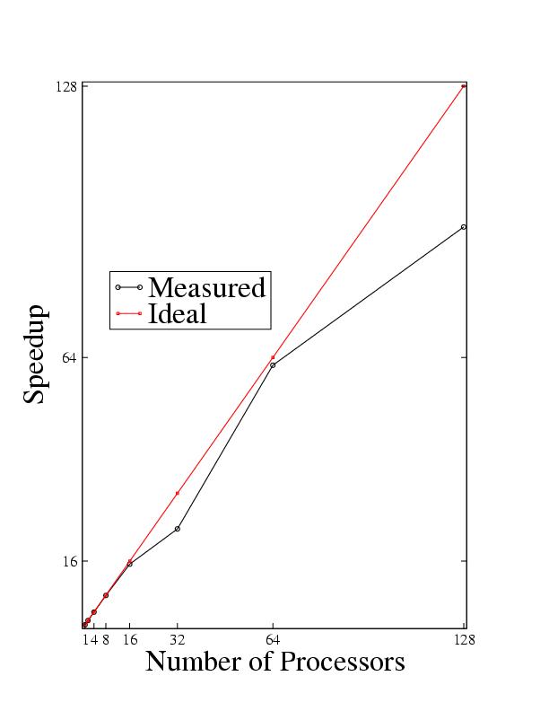
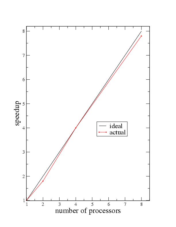This is a typical scaling for a 2-level mesh refined 3-D single black hole evolution. The black hole domain was -10M..10M with resolutions of 2.5 points/M and 5.0 points/M. The refinement region was from from -5M..5M ( M is the mass of the black hole ). The runs were performed on the Cray-Dell Linux Cluster at the Texas Advanced Computing Center . The code was compiled using the intel compilers. The system took 30 minutes to evolve ~100 steps on a single processor. Mesh refined elliptic solves were performed after evolution steps.

Speed-up defined:

speedup( m ) = completion time on one processor/ completion time on m processors.
For comparison, here are unigrid speedup results for the same code:

This is a typical scaling for a unigrid 3-D single black hole evolution. The black hole domain was -8M..8M with a resolution of 5 points/M. The system was evolved for 10M in time, requiring ~100 elliptic solves ( about 1 elliptic solve every 20 timesteps in this case ).

Compare unigrid and mesh refined memory requirements:

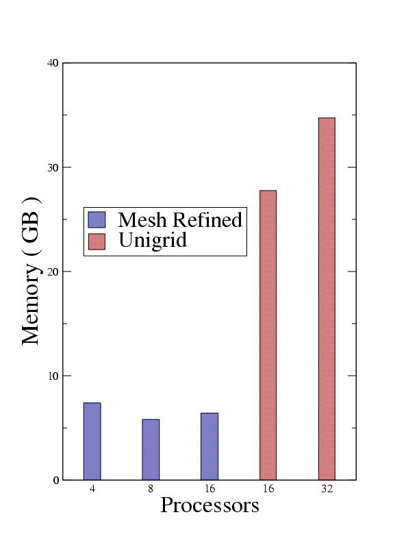Here are the memory requirements for a -20M..20M domain isolated black hole evolution. Keep in mind that to simulate gravitational radiation, domains of at least -100M..100M are necessary. The unigrid code has a resolution of 5 points/M throughout the entire domain. The mesh refined code has a resolution of 5 points/M from -5M..5M and 2.5 points/M for the global coarse mesh. The unigrid mesh was not performed on fewer than 16 processors because of insufficient memory.

Performance:
Compare unigrid and mesh refined performance:

Above is the a bar graph showing how far the code evolved ( in terms of M, the mass of the black hole ) in one real-time hour. The mesh refined case using 4 processors was able to equal the performance of 32 processors evolving the analogous unigrid case. Both give comparable results ( convergence tests are underway ). The mesh refined code on 16 processors ran 6.8 times faster than the unigrid case on 32 processors. The simulation in each case is a single isolated black hole on a domain of -20M..20M with the finest resolution at 5 points/M. Full Disclosure: This graph is a little misleading because the evolution scheme uses an adaptive timestep. This gives a speed-up later in the evolution that is not due to any parallelism ( e.g. the timesteps between 1 and 2 M are bigger than those between 0 and 1 M, regardless of the number of processors ).

Coming Soon...

Binary black hole evolutions and collisions using mesh refinement are on schedule for implementation. These simulations will involve adaptive mesh refinement.

Special thanks to Elijah Newren (Univ of Utah) and Thomas Adams (LLNL) for help critical to get this project underway